


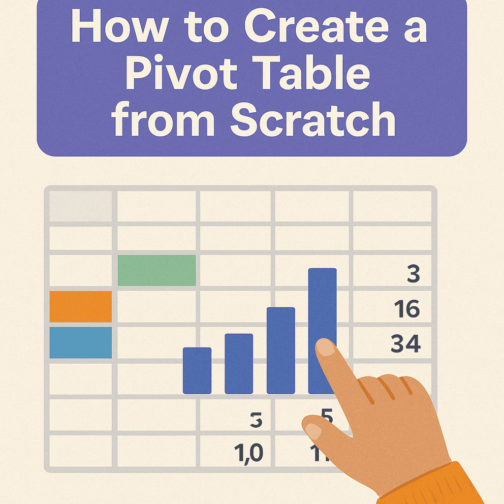
Creating a pivot table in Excel is a fantastic way to summarize and analyze data without excessive calculations. Let’s walk through it step by step, with real-world examples and a mini-case study to make it engaging. 😄
Imagine you’re a sales manager at a retail company. You have a dataset that tracks sales transactions, including columns for Date, Product, Customer, Region, and Amount. Here’s a simplified view of what your data might look like:
| Date | Product | Customer | Region | Amount |
|---|---|---|---|---|
| 2023-01-01 | Widget | Alice | North | $100 |
| 2023-01-02 | Gadget | Bob | South | $150 |
| 2023-01-01 | Widget | Charlie | East | $50 |
| 2023-01-03 | Gadget | Alice | North | $200 |
| 2023-01-03 | Widget | Bob | South | $120 |
With this data, you want to find out the total sales per product in each region.
Step 1: Prepare Your Data
Ensure your data is in a tabular format with headers. There should be no blank rows or columns. This forms the backbone of your pivot table.
Step 2: Insert a Pivot Table
- Select Your Data: Click anywhere inside your dataset.
- Go to the Insert Tab: Locate the Ribbon at the top of Excel and click on the “Insert” tab.
- Click on Pivot Table: In the options, find and click on the “Pivot Table” button.
A dialog box will appear asking where to place your pivot table. You can choose to put it in a new worksheet or an existing one. For this example, let’s place it in a new worksheet.
Step 3: Designing the Pivot Table
Once your pivot table is created, you’ll see the PivotTable Field List on the right side of the Excel window. This is where the magic happens!
- Drag Fields:
- Move “Product” to the Rows box.
- Move “Region” to the Columns box.
- Move “Amount” to the Values box.
Your pivot table will automatically calculate the total sales for each product in each region, presenting a clear overview:
| Product | North | South | East |
|---|---|---|---|
| Widget | $100 | $120 | $50 |
| Gadget | $200 | $150 | – |
💡 Tip: You can adjust the way values are summarized (like changing from Sum to Count) by clicking on the drop-down arrow next to “Sum of Amount” in the Values area.
Step 4: Customizing the Pivot Table
You can further customize your pivot table to make it more informative:
- Value Field Settings: Right-click on any value to change its summary function.
- Formatting: Select the cells in the pivot table, right-click, and select ‘Format Cells’ to apply currency formatting.
- Refresh Data: If your original data changes, you can refresh the pivot table by right-clicking it and selecting “Refresh.”
Step 5: Filtering and Slicing
Adding filters makes it easier to focus on specific data. By dragging the “Date” field to the Filters section, you can filter sales data by particular dates.
Alternatively, you can use a slicer for a more visual approach.
- Insert Slicer: Click on the Pivot Table Analyze tab, select “Insert Slicer,” and choose the fields you want to slice by (e.g., Product or Region).
- Click the buttons on the slicer to filter your data interactively!
Case Study Example: Analyzing Sales
Let’s consider an example. Say you want to prepare for a quarterly sales review. You can use the pivot table you created to showcase product performance across regions.
- Filter by Date: Select a specific month or quarter.
- Analyze: Present your findings to the team—like which products performed best in specific regions.
Your pivot analysis might reveal insights, such as:
- Widgets performed better in North and East regions compared to Gadgets.
- Product sales surged in the North during January.
Exporting and Sharing
Once your pivot table is done, you can share the worksheet with your team. Use Excel’s sharing features or simply send the file. To export, go to “File” > “Export” and choose your preferred format (like PDF or XLSX).
Conclusion
Creating a pivot table isn’t just about summarizing data; it’s about gaining insights and making data-driven decisions. Excel makes this process user-friendly, letting you explore your data in countless ways.
For more resources, check out:
FAQs
1. What if my data changes?
- You can refresh your pivot table by right-clicking on it and selecting “Refresh.”
2. Can I create multiple pivot tables from the same data?
- Yes, you can create as many pivot tables as you want from the same dataset.
3. What to do if my pivot table is blank?
- Check if your original data has any blank rows or columns and ensure your filters are set correctly.
4. Can I use pivot tables with large datasets?
- Yes, Excel handles large datasets well, but performance may vary based on your system’s capabilities.
5. Is there a way to visualize the data directly in projection?
- You can create pivot charts directly from your pivot tables by selecting “Pivot Chart” under the PivotTable Analyze tab.
Now you’re ready to dive into the world of pivot tables! Happy analyzing! 📊