



How to Use VLOOKUP Function in Excel: A Step-by-Step Guide
VLOOKUP, or “Vertical Lookup,” is one of Excel’s most useful functions and can save you tons of time when working with large data sets. Let’s walk through how to use this powerful feature step by step.
Understanding VLOOKUP
At its core, VLOOKUP helps you find a specific value in one column of a table, then retrieves a value from a different column in the same row. It’s handy for tasks such as merging data, finding specific information, and creating reports.
Here’s the basic syntax of the VLOOKUP function:
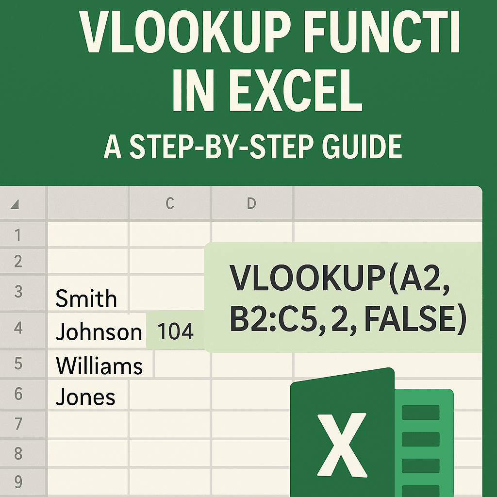
=VLOOKUP(lookup_value, table_array, col_index_num, [range_lookup])
- lookup_value: The value you want to search for.
- table_array: The range of cells that contains the data.
- col_index_num: The column number in the table from which to retrieve the value.
- [range_lookup]: Optional. TRUE for approximate match, FALSE for an exact match.
Step-by-Step Example
Let’s say you manage a store and have two tables: one with product IDs and names, and another with sales data. Your goal is to find the product name using the product ID from the sales table.
Sample Data
Products Table
| Product ID | Product Name |
|---|---|
| 101 | Apples |
| 102 | Bananas |
| 103 | Cherries |
| 104 | Dates |
Sales Table
| Sale ID | Product ID | Quantity |
|---|---|---|
| 001 | 101 | 10 |
| 002 | 103 | 5 |
| 003 | 102 | 7 |
Creating the Formula
-
Start in Sales Table: In the Sales Table, you’ll want to retrieve the Product Name. Let’s assume you want to put the Product Name in Column D next to Quantity. Click on cell D2.
-
Enter the VLOOKUP Formula: Type the following formula in D2:
=VLOOKUP(B2, $A$1:$B$5, 2, FALSE)
Here’s the breakdown:
- B2 is the Product ID you want to look up.
- $A$1:$B$5 is the range of the Products Table (make sure to adjust based on your actual table).
- 2 tells Excel to return the value from the second column of the range.
- FALSE means you want an exact match.
-
Drag to Fill: After entering the formula, click on the bottom-right corner of the cell (the fill handle) and drag it down to apply the formula to other cells in Column D.
Your Sales Table should now look like this:
| Sale ID | Product ID | Quantity | Product Name |
|---|---|---|---|
| 001 | 101 | 10 | Apples |
| 002 | 103 | 5 | Cherries |
| 003 | 102 | 7 | Bananas |
Tips for Using VLOOKUP
-
Table Array: Always ensure the ‘table_array’ includes the column that has your ‘lookup_value’ as the first column.
-
Exact Match: For most accurate results, use FALSE in the range_lookup to avoid unexpected outcomes.
-
Error Handling: To avoid #N/A errors when a lookup fails, consider wrapping your VLOOKUP in the IFERROR function:
=IFERROR(VLOOKUP(B2, $A$1:$B$5, 2, FALSE), “Not Found”)
Practical Case Study
Consider a situation where your business wants to track customer purchases effectively. You have a table with customer details (Customer ID, Name, and Email) and another table with their purchase history. By using VLOOKUP, you can aggregate all relevant data into one view.
Customer Table
| Customer ID | Customer Name | |
|---|---|---|
| C001 | John Doe | john@example.com |
| C002 | Jane Smith | jane@example.com |
| C003 | Mike Brown | mike@example.com |
Purchase History Table
| Purchase ID | Customer ID | Product |
|---|---|---|
| P001 | C001 | Laptops |
| P002 | C003 | Mobile Phones |
| P003 | C001 | Headphones |
You can use VLOOKUP to bring together all this information.
- In your Purchase History Table, create a new column called Customer Name.
- Use the VLOOKUP function to pull in the customer’s name from the Customer Table.
Final Thoughts
Using VLOOKUP effectively streamlines data management tasks, making it a go-to function for Excel users. The technique outlined above is just the beginning. VLOOKUP can be combined with other Excel functions for even more powerful data analysis.
For more Excel resources, check out:
FAQs
1. What if my lookup column is not the first column?
You can rearrange your data or consider using the INDEX-MATCH functions instead.
2. Can VLOOKUP handle multiple criteria?
No, VLOOKUP cannot directly handle multiple criteria. You may need to combine columns or explore more complex formulas (like INDEX-MATCH) or use helper columns.
3. What if my data changes frequently?
Always use a dynamic range (tables or named ranges) to accommodate data updates without changing your formulas.
4. Is there an alternative to VLOOKUP?
Yes! The INDEX-MATCH combination is a powerful alternative that is more flexible.
Feel free to explore more and let VLOOKUP make your data management task easier! 🎉