Earned schedule: turn progress into time
Calculate earned schedule from a planned-value curve, interpret time-based variance, and avoid misleading finish forecasts.
By Dr. Hassan Khames EliwaLast updated
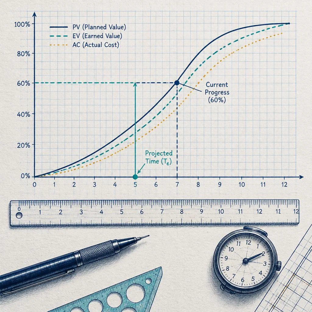
Ask when today's progress was supposed to exist
Earned schedule translates earned value into a position on the baseline timeline. It asks when the approved plan expected to achieve the amount of budgeted work actually completed. Comparing that earned time with actual elapsed time gives a schedule variance measured in time rather than money.
This makes a status conversation more direct. “We have earned five months of planned progress after six months” is easier to interpret than a currency-denominated schedule variance. It still describes aggregate progress, not the identity of the activities that control handover.
Use the earned schedule calculator with a cumulative planned-value series and the earned value at a common status date. The example below separates the measured result from the assumptions needed to forecast a finish.
Why ordinary SPI can lose its warning signal
Traditional earned value management uses planned value, PV, and earned value, EV. PV is the budgeted value of work scheduled by the status date. EV is the budgeted value of work actually accomplished. Neither is actual expenditure.
The conventional schedule performance index is EV / PV, and conventional schedule variance is EV − PV. Their units and interpretation follow budgeted work, even though their names refer to schedule.
At late completion, EV and PV both equal the total budget, assuming unchanged scope and a completed baseline. Conventional SPI therefore returns to 1 and schedule variance to zero, even if completion was months late. Walt Lipke's earned schedule method was developed to retain time-based schedule information, including at completion. 1
That limitation does not make conventional earned value useless. It means a cost-weighted progress indicator should not be mistaken for a direct measurement of elapsed delay.
Assemble a usable baseline curve
Our illustrative project has a budget at completion of $100,000 and a planned duration of eight months. Planned value is cumulative at each month-end, including a zero starting point.
| Elapsed month | Cumulative planned value |
|---|---|
| 0 | $0 |
| 1 | $5,000 |
| 2 | $15,000 |
| 3 | $30,000 |
| 4 | $50,000 |
| 5 | $70,000 |
| 6 | $85,000 |
| 7 | $95,000 |
| 8 | $100,000 |
At the end of month 6, verified earned value is $60,000. Keep this input tied to documented progress rules. For example, if equipment value is earned at delivery, a large shipment may create a progress jump without a comparable advance in installation readiness.
The baseline must use the same scope and valuation basis as EV. Mixing a revised budget curve with an old earned-value series can create a numerical result that has no coherent meaning.
Locate earned value on the time axis
The $60,000 earned value lies between planned values of $50,000 at month 4 and $70,000 at month 5. Four full baseline months have been earned, plus a fraction of the next interval.
The fraction is (60,000 − 50,000) / (70,000 − 50,000) = 10,000 / 20,000 = 0.5. Earned schedule, ES, is therefore 4.5 months.
For equally spaced intervals, the common expression is ES = C + (EV − PV at C) / (PV at C+1 − PV at C), where C is the last complete baseline interval reached. Lipke's concept paper explains this linear interpolation approach. 2
For unequal intervals, multiply the fraction by the actual interval width before adding it to the earlier time coordinate. A halfway value across a two-month interval earns one month, not half a month.
Calculate the time-based indicators
Actual time, AT, is six months. Time-based schedule variance is ES − AT = 4.5 − 6 = −1.5 months. Time-based schedule performance index is ES / AT = 4.5 / 6 = 0.75.
| Measure | Calculation | Result |
|---|---|---|
| Earned schedule | 4 + 10,000 / 20,000 | 4.5 months |
| Time variance, SV(t) | 4.5 − 6 | −1.5 months |
| Time index, SPI(t) | 4.5 / 6 | 0.75 |
| Conventional variance | 60,000 − 85,000 | −$25,000 |
| Conventional SPI | 60,000 / 85,000 | 0.7059 |
The time index says the project has earned 0.75 baseline months per elapsed month on average. It does not say every crew is working at 75% productivity. Different work packages, weighting rules and the shape of the baseline all contribute.
Likewise, the negative 1.5 months is an aggregate schedule position. It is not proof that the contractual finish will be exactly 1.5 months late.
Compare two explicit forecast assumptions
Suppose future progress proceeds at the baseline time efficiency of 1.0. Remaining earned time is planned duration minus earned schedule: 8 − 4.5 = 3.5 months. Adding that to actual time gives a forecast duration of 9.5 months.
Alternatively, assume the cumulative time efficiency of 0.75 persists. Forecast duration is 8 / 0.75 = 10.6667 months, or approximately 10.67 months. The equivalent remaining-duration calculation is 6 + (8 − 4.5) / 0.75.
These forecasts answer different questions. The first assumes recovery to planned efficiency for all remaining work; the second assumes continued cumulative efficiency. Neither incorporates a specific recovery action, seasonal shutdown or newly discovered dependency.
Do not add the full planned duration to actual time. Six months have already elapsed, and some baseline progress has already been earned. Forecast only the remaining portion under the chosen assumption.
Handle flat periods and boundary cases
A cumulative PV curve should not decline under a stable baseline. A flat interval is possible during a planned pause, but interpolation across a zero increase would divide by zero. Find an appropriate rising segment or report that the earned position is ambiguous across the plateau, using a documented convention.
At AT = 0, SPI(t) is undefined. When EV is zero, ES is normally zero under a baseline beginning at zero, but a planned initial idle period needs careful interpretation. Do not fabricate a positive efficiency merely to keep a dashboard green.
EV beyond the budget at completion, mismatched units or missing time coordinates should trigger investigation rather than silent extrapolation. Approved scope changes require a controlled baseline process and clear reporting of what changed.
Keep the critical-path review alongside the metric
Cost-weighted work is not evenly important to completion. An expensive noncritical delivery can improve EV while a low-budget approval blocks commissioning. Earned schedule can therefore improve while the likely finish deteriorates.
Ask which incomplete activities control the next milestone, whether their prerequisites are satisfied and whether resources can support the forecast. Compare the earned-schedule signal with the current network, not with a stale baseline bar chart alone.
A practical reporting cycle has three parts: validate physical progress, calculate the time indicators consistently, and explain the operational cause. “Behind because progress is low” is circular. “Testing access was lost for two weeks and the replacement window is unconfirmed” identifies something management can act on.
At completion after ten months, this example would have ES = 8, AT = 10, SV(t) = −2 months and SPI(t) = 0.8. Those values retain the late-finish signal that conventional SPI loses. Their value lies in a consistent time interpretation, not in replacing the detailed schedule that explains what happened.
Calculators used in this guide
Frequently asked questions
Is earned schedule measured in money?
No. It maps monetary or other budget-weighted earned value onto the baseline time axis, producing earned time in the units of that axis.
Does an SPI(t) below one mean the finish must be late?
It indicates aggregate progress behind the baseline time position. The eventual finish also depends on remaining critical work and future performance.
Can I interpolate across a flat planned-value interval?
Not using a zero denominator. Apply a documented plateau convention or identify the relevant rising interval and explain any ambiguity.
Why are the two example forecasts different?
The 9.5-month forecast assumes planned efficiency for remaining work. The 10.67-month forecast assumes cumulative time efficiency of 0.75 continues.
Does earned schedule replace a critical-path schedule?
No. It summarizes weighted progress in time units but does not identify the network activities or resource constraints controlling completion.
Sources and standards
About the author
Dr. Hassan Khames Eliwa holds a PhD in Construction & Built Environment and has more than 20 years of international project controls experience. He is Director of Eliwa Project Controls Limited in Auckland and founder of PMMilestone.org and PMMilestone.com.
Buy me a coffee