Monte Carlo schedule risk in plain English: what P50 and P80 actually mean
Read schedule percentiles without confusing a serial simulation, a network forecast and a commitment.
By Dr. Hassan Khames EliwaLast updated
P80 is a conditional forecast, not a promise
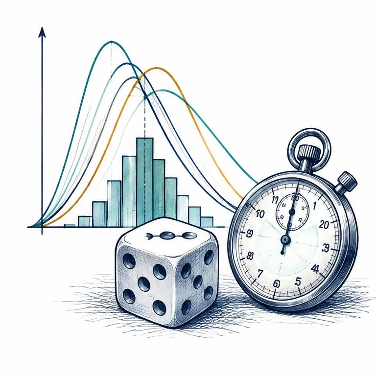
A P80 schedule duration is a point at or below which 80% of the modeled completion outcomes fall. P50 is the corresponding halfway point. Neither number says that the team has completed that percentage of the work, and neither creates a guarantee about the real project.
The qualification matters: these probabilities belong to a model with particular scope, logic, calendars and risk assumptions. Missing a permit dependency or assuming unlimited specialist crews can make a beautifully plotted distribution misleading. The useful question is not simply “What is P80?” It is “P80 of what model, under which conditions, and for which decision?”
Use the Monte Carlo risk calculator to explore duration uncertainty. This tool sums independent sequential rows; it does not simulate dependency networks, resource constraints or correlation. Treat its schedule output as a serial total, not automatically as a project finish forecast. Its interpolated percentile convention also differs from the nearest-rank teaching table below.
What the simulation repeatedly does
A duration simulation samples possible activity durations from specified distributions. For a genuinely sequential chain, each trial adds those sampled durations. Repeating the trial produces a collection of possible totals, which can be sorted to describe the modeled completion distribution.
A network simulation needs an additional step: recalculate the schedule through its dependency logic on every trial. At a merge point, a successor waits for all required predecessors, not for their durations to be added together. Different paths may control the finish in different trials.
Simulation does not discover uncertainty by itself. Estimators still choose distributions, ranges, dependencies and risk events. More trials can stabilize the numerical estimate for that chosen model; they cannot repair a missing scope item or a systematically optimistic estimating workshop.
Keep the distinction between working days and elapsed days explicit. A duration measured in working days becomes a calendar date only after applying a start date, working calendar, holidays and relevant availability rules.
Read percentiles from a deliberately hypothetical sample
The following table is a hypothetical ranked sample for teaching, not calculator output, a real forecast or the result of a Monte Carlo run. Its ten invented illustrative durations are chosen solely to make ranking visible. Use the nearest-rank convention: rank equals the percentile fraction multiplied by the sample count, rounded upward.
| Rank | Hypothetical total duration, working days | Interpretation |
|---|---|---|
| 1 | 10 | Shortest sample outcome |
| 2 | 11 | Two outcomes at or below 11 |
| 3 | 12 | Three outcomes at or below 12 |
| 4 | 13 | Four outcomes at or below 13 |
| 5 | 14 | P50 by nearest rank |
| 6 | 15 | Six outcomes at or below 15 |
| 7 | 16 | Seven outcomes at or below 16 |
| 8 | 18 | P80 by nearest rank |
| 9 | 21 | Nine outcomes at or below 21 |
| 10 | 25 | Longest sample outcome |
For P50, 0.50 × 10 gives rank 5, so the illustrative result is 14 working days. For P80, 0.80 × 10 gives rank 8, or 18 working days. Two of the ten sample outcomes are longer than 18 days.
The four-day difference between these illustrative percentiles is not a universal contingency rule. It belongs only to this teaching sample. Other percentile conventions interpolate between observations, so software can report slightly different values from the same finite sample. Ten outcomes are also far too few to treat this table as a robust risk analysis.
Separate the median from the average and the target
P50 is a median, not necessarily an average. A long unfavorable tail can pull the mean later than the median. The most likely single duration is another concept again: it describes the peak of a distribution, not its midpoint by cumulative probability.
A target date is a management choice. A contractual milestone is an obligation. A percentile is a description of modeled uncertainty. They can be compared, but should not share a label merely because someone wants one authoritative date on the dashboard.
If a chosen commitment corresponds to P80, the model still leaves an upper tail beyond it. Explain who bears that exposure, what mitigation remains available and which changes would require an updated analysis. Do not describe P80 as “80% certain” without stating the model assumptions and acknowledging that those assumptions can be wrong.
A serial PERT calculation is a useful cross-check
Consider two activities that must run one after another, without overlap. Each has optimistic, most likely and pessimistic durations of 2, 5 and 8 working days. The conventional PERT mean for each is (2 + 4 × 5 + 8) / 6 = 5 days. The conventional standard deviation approximation is (8 − 2) / 6 = 1 day.
Their expected serial total is 10 days. If the durations are independent, their variances add: 1² + 1² = 2 days squared, giving a combined standard deviation of approximately 1.414 days.
The PERT calculator can check these figures using its serial-task mode. Its normal-approximation percentile labels are not Monte Carlo results or exact quantiles of a bounded PERT distribution. The worked arithmetic here checks a mean and spread, not a claimed simulated P80.
Independence is needed for that simple variance addition, not for adding the expected durations of a fixed serial chain. With dependence, the total variance also includes covariance terms. That distinction prevents a common mistake: a plausible mean does not validate a narrow uncertainty range.
As a deterministic tool check, enter two rows with all three estimates fixed at 5 days. Every sequential trial must total 10 days, regardless of seed or distribution selection. This verifies addition only; zero-width inputs deliberately contain no modeled uncertainty and provide no evidence about real schedule confidence.
Parallel work changes the question
Suppose activities A and B can start together. A takes 6 days and B takes 8 days. Activity C takes 2 days and can start only after both finish. The deterministic network duration is max(6, 8) + 2 = 10 days, not 6 + 8 + 2 = 16 days.
Check this structure with the critical path and float calculator. This is a deterministic logic check, not a simulation. Its finish-start, zero-lag network assumptions must match the example being entered.
When durations become uncertain, A can sometimes overtake B as the controlling predecessor. The project duration in each trial is the longest required path through that trial's network. Simply simulating the currently critical path misses the possibility that another path becomes critical.
Resource restrictions add another complication. Two activities that appear parallel in the dependency graph may require the same crane or commissioning specialist. Unless the model represents that restriction, its apparent overlap is not a feasible execution plan.
Logic dependence and statistical correlation are different
A predecessor link says when an activity may start. Statistical correlation describes how uncertain outcomes tend to move together. A finish-start link does not automatically make durations correlated, and activities without a logic link can still share exposure to the same weather or supplier.
Positive correlation can widen the spread of a serial total relative to an independent model. In a network, its effect also depends on where shared exposures sit and which paths compete. Avoid a blanket percentage adjustment presented as a substitute for understanding those relationships.
Discrete events deserve explicit treatment. A permit rejection may occur or not occur; if it occurs, it may introduce a defined rework branch. Hiding that event inside every activity's pessimistic duration can double-count the same risk. Conversely, leaving it out of both activity ranges and the risk register excludes it altogether.
Turn a percentile into a decision record
Before presenting results, verify the status date, remaining scope, calendar basis and treatment of already completed work. Check missing predecessors, unjustified constraints and unrealistic overlap. The GAO Schedule Assessment Guide emphasizes a credible integrated schedule as the foundation for useful schedule risk analysis.
Then record the distribution assumptions, dependence treatment, simulation settings and percentile convention. Where a tool uses repeatable pseudo-random sampling, retain the seed when available. Compare repeated runs or larger trial counts to assess numerical stability, while recognizing that stable output can still come from a poor model.
Test an actionable response rather than merely selecting a later date. Securing an inspection slot or splitting a constrained work package changes specific assumptions that can be reviewed. A generic instruction to “work harder” does not define a defensible alternative model.
At the next reporting cycle, update remaining uncertainty using actual field evidence. Preserve the previous assumptions and explain why the forecast moved. That change record usually supports a better management conversation than another decimal place on P80.
Calculators used in this guide
Frequently asked questions
Does P80 guarantee the project will finish on time?
No. P80 describes a percentile of the modeled outcomes. Excluded risks, unrealistic logic and changed conditions can invalidate the forecast, and the model itself retains outcomes beyond P80.
Is P50 the average duration?
Not necessarily. P50 is the median. The mean can differ, especially when the completion distribution has a long unfavorable tail.
Can the Monte Carlo risk calculator model parallel paths?
No. Its schedule mode sums independent sequential rows. A network forecast requires dependency logic to be recalculated in every trial, with relevant resource restrictions and dependence represented.
Why does correlation matter?
Shared exposures can move multiple durations together. An independent model omits that relationship; for serial totals, positive correlation can widen the spread compared with independent sampling.
Why can two tools report different percentiles?
They may use different distributions, seeds, trial counts or percentile conventions. The hypothetical table uses nearest rank; the proposed calculator interpolates between sorted outcomes.
Sources and standards
About the author
Dr. Hassan Khames Eliwa holds a PhD in Construction & Built Environment and has more than 20 years of international project controls experience. He is Director of Eliwa Project Controls Limited in Auckland and founder of PMMilestone.org and PMMilestone.com.
Buy me a coffee